Getting Started 
CAX is a high-performance and flexible open-source library designed to accelerate artificial life research. 🧬

Abstract
Cellular automata have become a cornerstone for investigating emergence and self-organization across diverse scientific disciplines. However, the absence of a hardware-accelerated cellular automata library limits the exploration of new research directions, hinders collaboration, and impedes reproducibility. In this work, we introduce CAX (Cellular Automata Accelerated in JAX), a high-performance and flexible open-source library designed to accelerate cellular automata research. CAX delivers cutting-edge performance through hardware acceleration while maintaining flexibility through its modular architecture, intuitive API, and support for both discrete and continuous cellular automata in arbitrary dimensions. We demonstrate CAX's performance and flexibility through a wide range of benchmarks and applications. From classic models like elementary cellular automata and Conway's Game of Life to advanced applications such as growing neural cellular automata and self-classifying MNIST digits, CAX speeds up simulations up to 2,000 times faster. Furthermore, we demonstrate CAX's potential to accelerate research by presenting a collection of three novel cellular automata experiments, each implemented in just a few lines of code thanks to the library's modular architecture. Notably, we show that a simple one-dimensional cellular automaton can outperform GPT-4 on the 1D-ARC challenge.
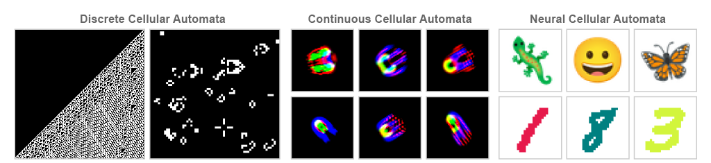
Cellular Automata
A cellular automaton is a simple model of computation consisting of a regular grid of cells, each in a particular state. The grid can be in any finite number of dimensions. For each cell, a set of cells called its neighborhood is defined relative to the specified cell. The grid is updated at discrete time steps according to a fixed rule that determines the new state of each cell based on its current state and the states of the cells in its neighborhood.
CAX Architecture
CAX introduces a unifying framework for all cellular automata types. This flexible architecture is built upon two key components: the perceive module and the update module. Together, these modules define the local rule of the CA. At each time step, this local rule is applied uniformly to all cells in the grid, generating the next global state of the system.
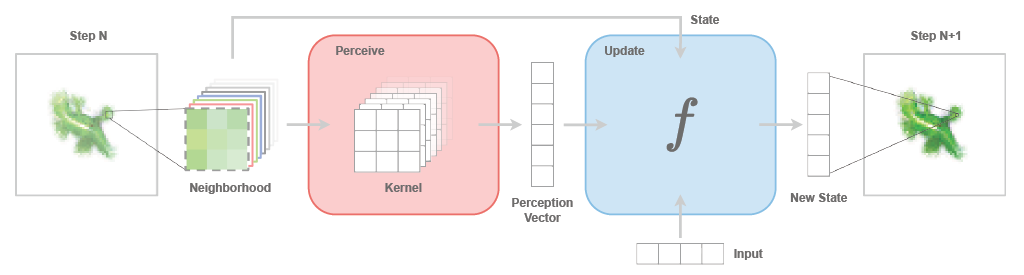
Figure adapted from "Growing Neural Cellular Automata", Mordvintsev et al. (2020), under CC-BY 4.0 license.
CAX's architecture introduces the novel concept of Controllable Cellular Automata that extend the capabilities of traditional CAs by making them responsive to external inputs, akin to recurrent neural networks processing sequential data, see Figure above. Controllable cellular automata bridge the gap between recurrent convolutional neural networks and cellular automata, opening up new possibilities for modeling complex systems that exhibit both autonomous emergent behavior and responsiveness to external control.
For CA experiments with external inputs, see examples/41_growing_conditional_nca.ipynb and examples/42_growing_unsupervised_nca.ipynb for example.
Let's dive in
In this notebook, we will explore how to use CAX to both:
- instantiate classic cellular automata like the Game of Life and
- create custom cellular automata from scratch.
You'll learn the fundamental concepts and implementation techniques that make CAX a powerful framework for cellular automata experimentation.
Installation
You will need Python 3.11 or later, and a working JAX installation. For example, you can install JAX with:
%pip install -U "jax[cuda]"
Then, install CAX from PyPi:
%pip install -U "cax[examples]"
Import
import jax
import jax.numpy as jnp
import mediapy
from flax import nnx

from cax.core import Input, State
Explore ready-to-use cellular automata
In this section, we'll demonstrate the basic usage of CAX with pre-implemented cellular automata. We'll instantiate Conway's Game of Life and visualize a glider pattern, showing how easily you can get started with existing systems in the library.
Configuration
First, we set up the configuration, including seed, spatial dimensions and the number of steps.
seed = 0

num_steps = 128
spatial_dims = (32, 32)

key = jax.random.key(seed)
rngs = nnx.Rngs(seed)
Instantiate system
Next, we instantiate Conway's Game of Life.
from cax.cs.life import Life

birth, survival = Life.birth_survival_from_string("B3/S23")
cs = Life(birth=birth, survival=survival, rngs=rngs)
nnx.display(cs)
Sample initial state
Then, we define a function to sample an initial state, which is essential for running a system.
def sample_state():
	"""Sample a state with a glider for the Game of Life."""
	state = jnp.zeros((*spatial_dims, 1))

	mid_x, mid_y = spatial_dims[0] // 2, spatial_dims[1] // 2
	glider = jnp.array(
		[
			[0.0, 1.0, 0.0],
			[0.0, 0.0, 1.0],
			[1.0, 1.0, 1.0],
		]
	)
	return state.at[mid_x : mid_x + 3, mid_y : mid_y + 3, 0].set(glider)
Run
Given an initial state and the system, we can simulate for num_steps.
state_init = sample_state()
state_final = cs(state_init, num_steps=num_steps, sow=True)
Visualize
We start from state_init sampled with our function sample_state, and then we apply the complex system cs for num_steps to get the state_final.
However, to visualize the evolution of the complex system, we need to have access to the intermediate states. But how do we do that?
To do that, we use the nnx.sow utilities from Flax. The sow mechanism allows you to collect intermediate values during computation by "sowing" them into a collection that can be retrieved later. For more details, see the official Flax documentation.
Implemented complex systems, such as Life, already offer the possibility to sow the intermediate states of the system during the evolution, and can be accessed with the cell below.
intermediates = nnx.pop(cs, nnx.Intermediate)
states = intermediates.state[0]
Now that we have the initial state state_init, as well as the intermediate states states, we can visualize the evolution of the complex system.
All complex systems must include a render method to convert a state into an RGB frame. For the Game of Life, a ready-to-use render method is provided, allowing you to easily generate a frame with a simple call: frame = cs.render(state).
Enjoy! 👾
states = jnp.concatenate([state_init[None], states])  # concatenate initial state with other states
frames = nnx.vmap(  # render each frame
	lambda cs, state: cs.render(state),
	in_axes=(None, 0),
)(cs, states)

mediapy.show_video(frames, width=256, height=256, codec="gif")
Custom metrics
While visualizing the evolution of states can produce captivating simulations, we often also want to track additional metrics to better understand how the system evolves over time.
By default, CAX enables to sow the states encountered during the system’s evolution. However, this behavior is highly customizable. In this section, we’ll explore how to create a tailored metrics function to sow custom metrics suited to your needs.
First, let's define a metrics function.
def metrics_fn(state, next_state, perception):
	"""Metrics function for the Game of Life."""
	neighbors_alive_count = perception[..., 1:2]
	return {
		"num_neighbors": jnp.mean(neighbors_alive_count),
		"growth_rate": jnp.sum(next_state) - jnp.sum(state),
	}
Then, we will need to create a custom Life class, that sow our desired metrics during the step function.
class CustomLife(Life):
	"""Custom Life class with custom metrics."""

	def _step(self, state: State, input: Input | None = None, *, sow: bool = False) -> State:
		perception = self.perceive(state)
		next_state = self.update(state, perception, input)

		if sow:
			metrics = metrics_fn(state, next_state, perception)
			self.sow(nnx.Intermediate, "state", next_state)
			self.sow(nnx.Intermediate, "metrics", metrics)

		return next_state
Let's instantiate the Game of Life with this custom metrics function.
cs = CustomLife(birth=birth, survival=survival, rngs=rngs)
This time, we will generate a state composed of randomly initialized cells, drawn from a Bernoulli distribution where each cell has a 0.1 probability of being alive.
def sample_state(key, p=0.1):
	"""Sample a random state for the Game of Life."""
	return jax.random.bernoulli(key, p=p, shape=(*spatial_dims, 1)).astype(jnp.float32)
Let's run the system:
key, subkey = jax.random.split(key)
state_init = sample_state(subkey)
state_final = cs(state_init, num_steps=num_steps, sow=True)
...and visualize:
intermediates = nnx.pop(cs, nnx.Intermediate)
states = intermediates.state[0]
metrics = intermediates.metrics[0]
states = jnp.concatenate([state_init[None], states])
frames = nnx.vmap(
	lambda cs, state: cs.render(state),
	in_axes=(None, 0),
)(cs, states)

mediapy.show_video(frames, width=256, height=256, codec="gif")
Let's also plot the number of alive neighbors and growth rate over time:
import matplotlib.pyplot as plt

# Plot the metrics
fig, axes = plt.subplots(1, 2, figsize=(8, 4))

axes[0].plot(metrics["num_neighbors"])
axes[0].set_title("Number of Neighbors Alive")
axes[0].set_xlabel("Time Step")
axes[0].set_ylabel("Number of Neighbors Alive")

axes[1].plot(metrics["growth_rate"])
axes[1].set_title("Growth Rate")
axes[1].set_xlabel("Time Step")
axes[1].set_ylabel("Growth Rate")

plt.tight_layout()
plt.show()
Running parallel simulations
When using nnx.Modules with rngs in the state, we need to use nnx.split_rngs to properly vectorize over rngs state across parallel operations. For Conway's Game of Life specifically, the system doesn't use randomness during execution, so we could use nnx.vmap directly. However, we'll demonstrate the more general approach with nnx.split_rngs below, which works for any systems that maintain rngs state.
num_simulations = 8

# Sample initial states
key, subkey = jax.random.split(key)
keys = jax.random.split(subkey, num_simulations)
state_init = jax.vmap(sample_state)(keys)

# Run independent simulations in parallel
state_axes = nnx.StateAxes({nnx.RngState: 0, nnx.Intermediate: 0, ...: None})
state_final = nnx.split_rngs(splits=num_simulations)(
	nnx.vmap(
		lambda cs, state_init: cs(state_init, num_steps=num_steps, sow=True),
		in_axes=(state_axes, 0),
	)
)(cs, state_init)
intermediates = nnx.pop(cs, nnx.Intermediate)
states = intermediates.state[0]
states.shape  # (num_simulations, num_steps, *spatial_dims, num_channels)
states = jnp.concatenate([state_init[:, None], states], axis=1)
frames = nnx.vmap(
	lambda cs, state: cs.render(state),
	in_axes=(None, 0),
)(cs, states)

mediapy.show_videos(frames, width=128, height=128, codec="gif")
Create your own complex system from scratch
In this section, we will build a custom complex system from scratch.
In CAX, every complex system must inherit from the ComplexSystem class and implement two required methods:
_step: Defines how the system evolves over one time steprender: Converts the system state into a visual representation
The _step method can perform any computation, but it must follow this signature: take a State as input, an optional Input, and return an updated State. Many complex systems (like cellular automata or particle systems) follow a common pattern where individual components (e.g., cells, particles, etc.) first perceive their local neighborhood, then update their state based on this perception and current state. For this reason, we recommend structuring the _step method into two phases:
- Perceive: Gather information from the neighborhood
- Update: Modify the state based on current state and perception
This structure is optional but helps organize the code clearly.
In the following example, we'll build a two-dimensional Neural Cellular Automaton (NCA) using CAX's pre-built Perceive and Update modules. Our NCA will feature:
- Convolutional perception to gather neighborhood information
- Residual update mechanisms for stable learning
Note that we won't be training this neural cellular automaton in the current notebook - we'll focus solely on its construction and architecture.
Since each NCA is unique, CAX does not offer pre-built, ready-to-use NCAs. However, it provides a versatile toolkit that empowers users to swiftly develop a custom cellular automaton suited to their specific experimental needs. In this section, we will explore how to efficiently create a neural cellular automaton using these tools.
Configuration
seed = 0

num_steps = 256
num_spatial_dims = 2
channel_size = 16

num_kernels = 3
hidden_size = 128
cell_dropout_rate = 0.5

key = jax.random.key(seed)
rngs = nnx.Rngs(seed)
Custom Neural Cellular Automata
The final step to create the cellular automata is to combine the perceive and update modules.
Optionally, we can create a custom CA class inheriting from the base CA class to implement a custom render method and more.
from cax.core import ComplexSystem
from cax.core.perceive import ConvPerceive
from cax.core.update import ResidualUpdate
from cax.utils import clip_and_uint8, rgba_to_rgb


class CustomNCA(ComplexSystem):
	"""Custom neural cellular automaton."""

	def __init__(self, *, rngs: nnx.Rngs):
		"""Initialize custom cellular automaton.

		Args:
			rngs: rngs key.

		"""
		# CAX provides a set of perceive modules.
		# In this notebook, we will use a simple convolution perceive module.
		self.perceive = ConvPerceive(
			channel_size=channel_size,  # Number of channels per cell in the grid
			perception_size=2 * channel_size,  # Number of channels per cell in the perception
			rngs=rngs,
		)

		# CAX provides a set of update modules.
		# In this notebook, we will use a residual MLP update module.
		self.update = ResidualUpdate(
			num_spatial_dims=2,  # Number of spatial dimensions
			channel_size=channel_size,  # Number of channels per cell in the grid
			perception_size=2 * channel_size,  # Number of channels per cell in the perception
			hidden_layer_sizes=(hidden_size,),  # Sizes of hidden layers in the MLP
			rngs=rngs,
		)

	def _step(self, state: State, input: Input | None = None, *, sow: bool = False) -> State:
		perception = self.perceive(state)
		next_state = self.update(state, perception, input)

		if sow:
			self.sow(nnx.Intermediate, "state", next_state)

		return next_state

	@nnx.jit
	def render(self, state):
		"""Render state to RGB."""
		rgba = state[..., -4:]
		rgb = rgba_to_rgb(rgba)

		# Clip values to valid range and convert to uint8
		return clip_and_uint8(rgb)
cs = CustomNCA(rngs=rngs)
Sample initial state
import PIL

from cax.utils.emoji import get_emoji

size = 40
pad_width = 16

emoji_pil = get_emoji("✨")
emoji_pil = emoji_pil.resize((size, size), resample=PIL.Image.Resampling.LANCZOS)

y = jnp.array(emoji_pil, dtype=jnp.float32) / 255.0
y = jnp.pad(y, ((pad_width, pad_width), (pad_width, pad_width), (0, 0)))

mediapy.show_image(y)
def sample_state(y):
	"""Sample a state with the target image."""
	state_shape = y.shape[:2] + (channel_size,)
	state = jnp.zeros(state_shape)

	# Set the target image in the RGB channels
	return state.at[:, :, :4].set(y)
Visualize
Run the cellular automata for 256 steps.
state_init = sample_state(y)
state_final = cs(state_init, num_steps=num_steps, sow=True)
Clip the states to display as a video.
intermediates = nnx.pop(cs, nnx.Intermediate)
states = intermediates.state[0]
states = jnp.clip(jnp.concatenate([state_init[None], states]), min=0.0, max=1.0)
Now you know how to run cellular automata with CAX! Go through the other notebooks to understand how to run classic cellular automata such as Game of Life or Lenia, or train neural cellular automata such as growing neural cellular automata.
frames = nnx.vmap(
	lambda cs, state: cs.render(state),
	in_axes=(None, 0),
)(cs, states)

mediapy.show_video(frames, width=256, height=256, codec="gif")